\(\kappa\)-Stereographic Projection model
Stereographic projection models comes to bind constant curvature spaces. Such as spheres, hyperboloids and regular Euclidean manifold. Let’s look at what does this mean. As we mentioned constant curvature, let’s name this constant \(\kappa\).
Hyperbolic spaces
Hyperbolic space is a constant negative curvature (\(\kappa < 0\)) Riemannian manifold. (A very simple example of Riemannian manifold with constant, but positive curvature is sphere, we’ll be back to it later)
An (N+1)-dimensional hyperboloid spans the manifold that can be embedded into N-dimensional space via projections.
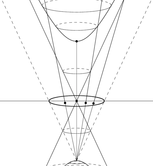
Originally, the distance between points on the hyperboloid is defined as
Not to work with this manifold, it is convenient to project the hyperboloid onto a plane. We can do it in many ways recovering embedded manifolds with different properties (usually numerical). To connect constant curvature manifolds we better use Poincare ball model (aka stereographic projection model).
Poincare Model
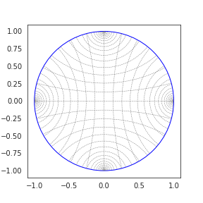
Grid of Geodesics for \(\kappa=-1\), credits to Andreas Bloch
First of all we note, that Poincare ball is embedded in a Sphere of radius \(r=1/\sqrt{\kappa}\), where c is negative curvature. We also note, as \(\kappa\) goes to \(0\), we recover infinite radius ball. We should expect this limiting behaviour recovers Euclidean geometry.
Spherical Spaces
Another case of constant curvature manifolds is sphere. Unlike Hyperboloid this manifold is compact and has positive \(\kappa\). But still we can embed a sphere onto a plane ignoring one of the poles.
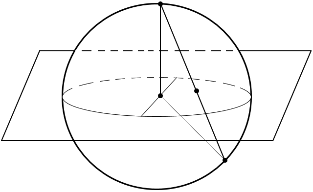
Once we project sphere on the plane we have the following geodesics
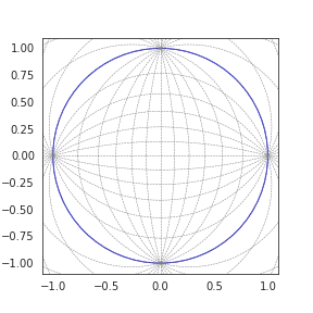
Grid of Geodesics for \(\kappa=1\), credits to Andreas Bloch
Again, similarly to Poincare ball case, we have Euclidean geometry limiting \(\kappa\) to \(0\).
Universal Curvature Manifold
To connect Euclidean space with its embedded manifold we need to get \(g^\kappa_x\). It is done via conformal factor \(\lambda^\kappa_x\). Note, that the metric tensor is conformal, which means all angles between tangent vectors are remained the same compared to what we calculate ignoring manifold structure.
The functions for the mathematics in gyrovector spaces are taken from the following resources:
- [1] Ganea, Octavian, Gary Bécigneul, and Thomas Hofmann. “Hyperbolic
- neural networks.” Advances in neural information processing systems. 2018.
- [2] Bachmann, Gregor, Gary Bécigneul, and Octavian-Eugen Ganea. “Constant
- Curvature Graph Convolutional Networks.” arXiv preprint arXiv:1911.05076 (2019).
- [3] Skopek, Ondrej, Octavian-Eugen Ganea, and Gary Bécigneul.
- “Mixed-curvature Variational Autoencoders.” arXiv preprint arXiv:1911.08411 (2019).
- [4] Ungar, Abraham A. Analytic hyperbolic geometry: Mathematical
- foundations and applications. World Scientific, 2005.
- [5] Albert, Ungar Abraham. Barycentric calculus in Euclidean and
- hyperbolic geometry: A comparative introduction. World Scientific, 2010.
-
geoopt.manifolds.stereographic.math.lambda_x(x: torch.Tensor, *, k: torch.Tensor, keepdim=False, dim=-1)[source]¶ Compute the conformal factor \(\lambda^\kappa_x\) for a point on the ball.
\[\lambda^\kappa_x = \frac{2}{1 + \kappa \|x\|_2^2}\]Parameters: Returns: conformal factor
Return type: tensor
\(\lambda^\kappa_x\) connects Euclidean inner product with Riemannian one
-
geoopt.manifolds.stereographic.math.inner(x: torch.Tensor, u: torch.Tensor, v: torch.Tensor, *, k, keepdim=False, dim=-1)[source]¶ Compute inner product for two vectors on the tangent space w.r.t Riemannian metric on the Poincare ball.
\[\langle u, v\rangle_x = (\lambda^\kappa_x)^2 \langle u, v \rangle\]Parameters: Returns: inner product
Return type: tensor
-
geoopt.manifolds.stereographic.math.norm(x: torch.Tensor, u: torch.Tensor, *, k: torch.Tensor, keepdim=False, dim=-1)[source]¶ Compute vector norm on the tangent space w.r.t Riemannian metric on the Poincare ball.
\[\|u\|_x = \lambda^\kappa_x \|u\|_2\]Parameters: Returns: norm of vector
Return type: tensor
-
geoopt.manifolds.stereographic.math.egrad2rgrad(x: torch.Tensor, grad: torch.Tensor, *, k: torch.Tensor, dim=-1)[source]¶ Convert the Euclidean gradient to the Riemannian gradient.
\[\nabla_x = \nabla^E_x / (\lambda_x^\kappa)^2\]Parameters: - x (tensor) – point on the manifold
- grad (tensor) – Euclidean gradient for \(x\)
- k (tensor) – sectional curvature of manifold
- dim (int) – reduction dimension for operations
Returns: Riemannian gradient \(u\in T_x\mathcal{M}_\kappa^n\)
Return type: tensor
Math
The good thing about Poincare ball is that it forms a Gyrogroup. Minimal definition of a Gyrogroup assumes a binary operation \(*\) defined that satisfies a set of properties.
- Left identity
- For every element \(a\in G\) there exist \(e\in G\) such that \(e * a = a\).
- Left Inverse
- For every element \(a\in G\) there exist \(b\in G\) such that \(b * a = e\)
- Gyroassociativity
- For any \(a,b,c\in G\) there exist \(gyr[a, b]c\in G\) such that \(a * (b * c)=(a * b) * gyr[a, b]c\)
- Gyroautomorphism
- \(gyr[a, b]\) is a magma automorphism in G
- Left loop
- \(gyr[a, b] = gyr[a * b, b]\)
As mentioned above, hyperbolic space forms a Gyrogroup equipped with
-
geoopt.manifolds.stereographic.math.mobius_add(x: torch.Tensor, y: torch.Tensor, *, k: torch.Tensor, dim=-1)[source]¶ Compute the Möbius gyrovector addition.
\[x \oplus_\kappa y = \frac{ (1 - 2 \kappa \langle x, y\rangle - \kappa \|y\|^2_2) x + (1 + \kappa \|x\|_2^2) y }{ 1 - 2 \kappa \langle x, y\rangle + \kappa^2 \|x\|^2_2 \|y\|^2_2 }\]In general this operation is not commutative:
\[x \oplus_\kappa y \ne y \oplus_\kappa x\]But in some cases this property holds:
- zero vector case
\[\mathbf{0} \oplus_\kappa x = x \oplus_\kappa \mathbf{0}\]- zero curvature case that is same as Euclidean addition
\[x \oplus_0 y = y \oplus_0 x\]Another useful property is so called left-cancellation law:
\[(-x) \oplus_\kappa (x \oplus_\kappa y) = y\]Parameters: - x (tensor) – point on the manifold
- y (tensor) – point on the manifold
- k (tensor) – sectional curvature of manifold
- dim (int) – reduction dimension for operations
Returns: the result of the Möbius addition
Return type: tensor
-
geoopt.manifolds.stereographic.math.gyration(a: torch.Tensor, b: torch.Tensor, u: torch.Tensor, *, k: torch.Tensor, dim=-1)[source]¶ Compute the gyration of \(u\) by \([a,b]\).
The gyration is a special operation of gyrovector spaces. The gyrovector space addition operation \(\oplus_\kappa\) is not associative (as mentioned in
mobius_add()), but it is gyroassociative, which means\[u \oplus_\kappa (v \oplus_\kappa w) = (u\oplus_\kappa v) \oplus_\kappa \operatorname{gyr}[u, v]w,\]where
\[\operatorname{gyr}[u, v]w = \ominus (u \oplus_\kappa v) \oplus (u \oplus_\kappa (v \oplus_\kappa w))\]We can simplify this equation using the explicit formula for the Möbius addition [1]. Recall,
\[ \begin{align}\begin{aligned}\begin{split}A = - \kappa^2 \langle u, w\rangle \langle v, v\rangle - \kappa \langle v, w\rangle + 2 \kappa^2 \langle u, v\rangle \langle v, w\rangle\\ B = - \kappa^2 \langle v, w\rangle \langle u, u\rangle + \kappa \langle u, w\rangle\\ D = 1 - 2 \kappa \langle u, v\rangle + \kappa^2 \langle u, u\rangle \langle v, v\rangle\\\end{split}\\\operatorname{gyr}[u, v]w = w + 2 \frac{A u + B v}{D}.\end{aligned}\end{align} \]Parameters: - a (tensor) – first point on manifold
- b (tensor) – second point on manifold
- u (tensor) – vector field for operation
- k (tensor) – sectional curvature of manifold
- dim (int) – reduction dimension for operations
Returns: the result of automorphism
Return type: tensor
References
[1] A. A. Ungar (2009), A Gyrovector Space Approach to Hyperbolic Geometry
Using this math, it is possible to define another useful operations
-
geoopt.manifolds.stereographic.math.mobius_sub(x: torch.Tensor, y: torch.Tensor, *, k: torch.Tensor, dim=-1)[source]¶ Compute the Möbius gyrovector subtraction.
The Möbius subtraction can be represented via the Möbius addition as follows:
\[x \ominus_\kappa y = x \oplus_\kappa (-y)\]Parameters: - x (tensor) – point on manifold
- y (tensor) – point on manifold
- k (tensor) – sectional curvature of manifold
- dim (int) – reduction dimension for operations
Returns: the result of the Möbius subtraction
Return type: tensor
-
geoopt.manifolds.stereographic.math.mobius_scalar_mul(r: torch.Tensor, x: torch.Tensor, *, k: torch.Tensor, dim=-1)[source]¶ Compute the Möbius scalar multiplication.
\[r \otimes_\kappa x = \tan_\kappa(r\tan_\kappa^{-1}(\|x\|_2))\frac{x}{\|x\|_2}\]This operation has properties similar to the Euclidean scalar multiplication
- n-addition property
\[r \otimes_\kappa x = x \oplus_\kappa \dots \oplus_\kappa x\]- Distributive property
\[(r_1 + r_2) \otimes_\kappa x = r_1 \otimes_\kappa x \oplus r_2 \otimes_\kappa x\]- Scalar associativity
\[(r_1 r_2) \otimes_\kappa x = r_1 \otimes_\kappa (r_2 \otimes_\kappa x)\]- Monodistributivity
\[r \otimes_\kappa (r_1 \otimes x \oplus r_2 \otimes x) = r \otimes_\kappa (r_1 \otimes x) \oplus r \otimes (r_2 \otimes x)\]- Scaling property
\[|r| \otimes_\kappa x / \|r \otimes_\kappa x\|_2 = x/\|x\|_2\]Parameters: - r (tensor) – scalar for multiplication
- x (tensor) – point on manifold
- k (tensor) – sectional curvature of manifold
- dim (int) – reduction dimension for operations
Returns: the result of the Möbius scalar multiplication
Return type: tensor
-
geoopt.manifolds.stereographic.math.mobius_pointwise_mul(w: torch.Tensor, x: torch.Tensor, *, k: torch.Tensor, dim=-1)[source]¶ Compute the generalization for point-wise multiplication in gyrovector spaces.
The Möbius pointwise multiplication is defined as follows
\[\operatorname{diag}(w) \otimes_\kappa x = \tan_\kappa\left( \frac{\|\operatorname{diag}(w)x\|_2}{x}\tanh^{-1}(\|x\|_2) \right)\frac{\|\operatorname{diag}(w)x\|_2}{\|x\|_2}\]Parameters: - w (tensor) – weights for multiplication (should be broadcastable to x)
- x (tensor) – point on manifold
- k (tensor) – sectional curvature of manifold
- dim (int) – reduction dimension for operations
Returns: Möbius point-wise mul result
Return type: tensor
-
geoopt.manifolds.stereographic.math.mobius_matvec(m: torch.Tensor, x: torch.Tensor, *, k: torch.Tensor, dim=-1)[source]¶ Compute the generalization of matrix-vector multiplication in gyrovector spaces.
The Möbius matrix vector operation is defined as follows:
\[M \otimes_\kappa x = \tan_\kappa\left( \frac{\|Mx\|_2}{\|x\|_2}\tan_\kappa^{-1}(\|x\|_2) \right)\frac{Mx}{\|Mx\|_2}\]Parameters: - m (tensor) – matrix for multiplication. Batched matmul is performed if
m.dim() > 2, but only last dim reduction is supported - x (tensor) – point on manifold
- k (tensor) – sectional curvature of manifold
- dim (int) – reduction dimension for operations
Returns: Möbius matvec result
Return type: tensor
- m (tensor) – matrix for multiplication. Batched matmul is performed if
-
geoopt.manifolds.stereographic.math.mobius_fn_apply(fn: callable, x: torch.Tensor, *args, k: torch.Tensor, dim=-1, **kwargs)[source]¶ Compute the generalization of function application in gyrovector spaces.
First, a gyrovector is mapped to the tangent space (first-order approx.) via \(\operatorname{log}^\kappa_0\) and then the function is applied to the vector in the tangent space. The resulting tangent vector is then mapped back with \(\operatorname{exp}^\kappa_0\).
\[f^{\otimes_\kappa}(x) = \operatorname{exp}^\kappa_0(f(\operatorname{log}^\kappa_0(y)))\]Parameters: - x (tensor) – point on manifold
- fn (callable) – function to apply
- k (tensor) – sectional curvature of manifold
- dim (int) – reduction dimension for operations
Returns: Result of function in hyperbolic space
Return type: tensor
-
geoopt.manifolds.stereographic.math.mobius_fn_apply_chain(x: torch.Tensor, *fns, k: torch.Tensor, dim=-1)[source]¶ Compute the generalization of sequential function application in gyrovector spaces.
First, a gyrovector is mapped to the tangent space (first-order approx.) via \(\operatorname{log}^\kappa_0\) and then the sequence of functions is applied to the vector in the tangent space. The resulting tangent vector is then mapped back with \(\operatorname{exp}^\kappa_0\).
\[f^{\otimes_\kappa}(x) = \operatorname{exp}^\kappa_0(f(\operatorname{log}^\kappa_0(y)))\]The definition of mobius function application allows chaining as
\[y = \operatorname{exp}^\kappa_0(\operatorname{log}^\kappa_0(y))\]Resulting in
\[(f \circ g)^{\otimes_\kappa}(x) = \operatorname{exp}^\kappa_0( (f \circ g) (\operatorname{log}^\kappa_0(y)) )\]Parameters: - x (tensor) – point on manifold
- fns (callable[]) – functions to apply
- k (tensor) – sectional curvature of manifold
- dim (int) – reduction dimension for operations
Returns: Apply chain result
Return type: tensor
Manifold
Now we are ready to proceed with studying distances, geodesics, exponential maps and more
-
geoopt.manifolds.stereographic.math.dist(x: torch.Tensor, y: torch.Tensor, *, k: torch.Tensor, keepdim=False, dim=-1)[source]¶ Compute the geodesic distance between \(x\) and \(y\) on the manifold.
\[d_\kappa(x, y) = 2\tan_\kappa^{-1}(\|(-x)\oplus_\kappa y\|_2)\]Parameters: Returns: geodesic distance between \(x\) and \(y\)
Return type: tensor
-
geoopt.manifolds.stereographic.math.dist2plane(x: torch.Tensor, p: torch.Tensor, a: torch.Tensor, *, k: torch.Tensor, keepdim=False, signed=False, scaled=False, dim=-1)[source]¶ Geodesic distance from \(x\) to a hyperplane \(H_{a, b}\).
The hyperplane is such that its set of points is orthogonal to \(a\) and contains \(p\).
To form an intuition what is a hyperplane in gyrovector spaces, let’s first consider an Euclidean hyperplane
\[H_{a, b} = \left\{ x \in \mathbb{R}^n\;:\;\langle x, a\rangle - b = 0 \right\},\]where \(a\in \mathbb{R}^n\backslash \{\mathbf{0}\}\) and \(b\in \mathbb{R}^n\).
This formulation of a hyperplane is hard to generalize, therefore we can rewrite \(\langle x, a\rangle - b\) utilizing orthogonal completion. Setting any \(p\) s.t. \(b=\langle a, p\rangle\) we have
\[\begin{split}H_{a, b} = \left\{ x \in \mathbb{R}^n\;:\;\langle x, a\rangle - b = 0 \right\}\\ =H_{a, \langle a, p\rangle} = \tilde{H}_{a, p}\\ = \left\{ x \in \mathbb{R}^n\;:\;\langle x, a\rangle - \langle a, p\rangle = 0 \right\}\\ =\left\{ x \in \mathbb{R}^n\;:\;\langle -p + x, a\rangle = 0 \right\}\\ = p + \{a\}^\perp\end{split}\]Naturally we have a set \(\{a\}^\perp\) with applied \(+\) operator to each element. Generalizing a notion of summation to the gyrovector space we replace \(+\) with \(\oplus_\kappa\).
Next, we should figure out what is \(\{a\}^\perp\) in the gyrovector space.
First thing that we should acknowledge is that notion of orthogonality is defined for vectors in tangent spaces. Let’s consider now \(p\in \mathcal{M}_\kappa^n\) and \(a\in T_p\mathcal{M}_\kappa^n\backslash \{\mathbf{0}\}\).
Slightly deviating from traditional notation let’s write \(\{a\}_p^\perp\) highlighting the tight relationship of \(a\in T_p\mathcal{M}_\kappa^n\backslash \{\mathbf{0}\}\) with \(p \in \mathcal{M}_\kappa^n\). We then define
\[\{a\}_p^\perp := \left\{ z\in T_p\mathcal{M}_\kappa^n \;:\; \langle z, a\rangle_p = 0 \right\}\]Recalling that a tangent vector \(z\) for point \(p\) yields \(x = \operatorname{exp}^\kappa_p(z)\) we rewrite the above equation as
\[\{a\}_p^\perp := \left\{ x\in \mathcal{M}_\kappa^n \;:\; \langle \operatorname{log}_p^\kappa(x), a\rangle_p = 0 \right\}\]This formulation is something more pleasant to work with. Putting all together
\[\begin{split}\tilde{H}_{a, p}^\kappa = p + \{a\}^\perp_p\\ = \left\{ x \in \mathcal{M}_\kappa^n\;:\;\langle \operatorname{log}^\kappa_p(x), a\rangle_p = 0 \right\} \\ = \left\{ x \in \mathcal{M}_\kappa^n\;:\;\langle -p \oplus_\kappa x, a\rangle = 0 \right\}\end{split}\]To compute the distance \(d_\kappa(x, \tilde{H}_{a, p}^\kappa)\) we find
\[\begin{split}d_\kappa(x, \tilde{H}_{a, p}^\kappa) = \inf_{w\in \tilde{H}_{a, p}^\kappa} d_\kappa(x, w)\\ = \sin^{-1}_\kappa\left\{ \frac{ 2 |\langle(-p)\oplus_\kappa x, a\rangle| }{ (1+\kappa\|(-p)\oplus_\kappa \|x\|^2_2)\|a\|_2 } \right\}\end{split}\]Parameters: - x (tensor) – point on manifold to compute distance for
- a (tensor) – hyperplane normal vector in tangent space of \(p\)
- p (tensor) – point on manifold lying on the hyperplane
- k (tensor) – sectional curvature of manifold
- keepdim (bool) – retain the last dim? (default: false)
- signed (bool) – return signed distance
- scaled (bool) – scale distance by tangent norm
- dim (int) – reduction dimension for operations
Returns: distance to the hyperplane
Return type: tensor
-
geoopt.manifolds.stereographic.math.parallel_transport(x: torch.Tensor, y: torch.Tensor, v: torch.Tensor, *, k: torch.Tensor, dim=-1)[source]¶ Compute the parallel transport of \(v\) from \(x\) to \(y\).
The parallel transport is essential for adaptive algorithms on Riemannian manifolds. For gyrovector spaces the parallel transport is expressed through the gyration.
To recover parallel transport we first need to study isomorphisms between gyrovectors and vectors. The reason is that originally, parallel transport is well defined for gyrovectors as
\[P_{x\to y}(z) = \operatorname{gyr}[y, -x]z,\]where \(x,\:y,\:z \in \mathcal{M}_\kappa^n\) and \(\operatorname{gyr}[a, b]c = \ominus (a \oplus_\kappa b) \oplus_\kappa (a \oplus_\kappa (b \oplus_\kappa c))\)
But we want to obtain parallel transport for vectors, not for gyrovectors. The blessing is the isomorphism mentioned above. This mapping is given by
\[U^\kappa_p \: : \: T_p\mathcal{M}_\kappa^n \to \mathbb{G} = v \mapsto \lambda^\kappa_p v\]Finally, having the points \(x,\:y \in \mathcal{M}_\kappa^n\) and a tangent vector \(u\in T_x\mathcal{M}_\kappa^n\) we obtain
\[\begin{split}P^\kappa_{x\to y}(v) = (U^\kappa_y)^{-1}\left(\operatorname{gyr}[y, -x] U^\kappa_x(v)\right)\\ = \operatorname{gyr}[y, -x] v \lambda^\kappa_x / \lambda^\kappa_y\end{split}\]Parameters: - x (tensor) – starting point
- y (tensor) – end point
- v (tensor) – tangent vector at x to be transported to y
- k (tensor) – sectional curvature of manifold
- dim (int) – reduction dimension for operations
Returns: transported vector
Return type: tensor
-
geoopt.manifolds.stereographic.math.geodesic(t: torch.Tensor, x: torch.Tensor, y: torch.Tensor, *, k: torch.Tensor, dim=-1)[source]¶ Compute the point on the path connecting \(x\) and \(y\) at time \(x\).
The path can also be treated as an extension of the line segment to an unbounded geodesic that goes through \(x\) and \(y\). The equation of the geodesic is given as:
\[\gamma_{x\to y}(t) = x \oplus_\kappa t \otimes_\kappa ((-x) \oplus_\kappa y)\]The properties of the geodesic are the following:
\[\begin{split}\gamma_{x\to y}(0) = x\\ \gamma_{x\to y}(1) = y\\ \dot\gamma_{x\to y}(t) = v\end{split}\]Furthermore, the geodesic also satisfies the property of local distance minimization:
\[d_\kappa(\gamma_{x\to y}(t_1), \gamma_{x\to y}(t_2)) = v|t_1-t_2|\]“Natural parametrization” of the curve ensures unit speed geodesics which yields the above formula with \(v=1\).
However, we can always compute the constant speed \(v\) from the points that the particular path connects:
\[v = d_\kappa(\gamma_{x\to y}(0), \gamma_{x\to y}(1)) = d_\kappa(x, y)\]Parameters: - t (tensor) – travelling time
- x (tensor) – starting point on manifold
- y (tensor) – target point on manifold
- k (tensor) – sectional curvature of manifold
- dim (int) – reduction dimension for operations
Returns: point on the geodesic going through x and y
Return type: tensor
-
geoopt.manifolds.stereographic.math.geodesic_unit(t: torch.Tensor, x: torch.Tensor, u: torch.Tensor, *, k: torch.Tensor, dim=-1)[source]¶ Compute the point on the unit speed geodesic.
The point on the unit speed geodesic at time \(t\), starting from \(x\) with initial direction \(u/\|u\|_x\) is computed as follows:
\[\gamma_{x,u}(t) = x\oplus_\kappa \tan_\kappa(t/2) \frac{u}{\|u\|_2}\]Parameters: - t (tensor) – travelling time
- x (tensor) – initial point on manifold
- u (tensor) – initial direction in tangent space at x
- k (tensor) – sectional curvature of manifold
- dim (int) – reduction dimension for operations
Returns: the point on the unit speed geodesic
Return type: tensor
-
geoopt.manifolds.stereographic.math.expmap(x: torch.Tensor, u: torch.Tensor, *, k: torch.Tensor, dim=-1)[source]¶ Compute the exponential map of \(u\) at \(x\).
The expmap is tightly related with
geodesic(). Intuitively, the expmap represents a smooth travel along a geodesic from the starting point \(x\), into the initial direction \(u\) at speed \(\|u\|_x\) for the duration of one time unit. In formulas one can express this as the travel along the curve \(\gamma_{x, u}(t)\) such that\[\begin{split}\gamma_{x, u}(0) = x\\ \dot\gamma_{x, u}(0) = u\\ \|\dot\gamma_{x, u}(t)\|_{\gamma_{x, u}(t)} = \|u\|_x\end{split}\]The existence of this curve relies on uniqueness of the differential equation solution, that is local. For the universal manifold the solution is well defined globally and we have.
\[\begin{split}\operatorname{exp}^\kappa_x(u) = \gamma_{x, u}(1) = \\ x\oplus_\kappa \tan_\kappa(\|u\|_x/2) \frac{u}{\|u\|_2}\end{split}\]Parameters: - x (tensor) – starting point on manifold
- u (tensor) – speed vector in tangent space at x
- k (tensor) – sectional curvature of manifold
- dim (int) – reduction dimension for operations
Returns: \(\gamma_{x, u}(1)\) end point
Return type: tensor
-
geoopt.manifolds.stereographic.math.expmap0(u: torch.Tensor, *, k: torch.Tensor, dim=-1)[source]¶ Compute the exponential map of \(u\) at the origin \(0\).
\[\operatorname{exp}^\kappa_0(u) = \tan_\kappa(\|u\|_2/2) \frac{u}{\|u\|_2}\]Parameters: - u (tensor) – speed vector on manifold
- k (tensor) – sectional curvature of manifold
- dim (int) – reduction dimension for operations
Returns: \(\gamma_{0, u}(1)\) end point
Return type: tensor
-
geoopt.manifolds.stereographic.math.logmap(x: torch.Tensor, y: torch.Tensor, *, k: torch.Tensor, dim=-1)[source]¶ Compute the logarithmic map of \(y\) at \(x\).
\[\operatorname{log}^\kappa_x(y) = \frac{2}{\lambda_x^\kappa} \tan_\kappa^{-1}(\|(-x)\oplus_\kappa y\|_2) * \frac{(-x)\oplus_\kappa y}{\|(-x)\oplus_\kappa y\|_2}\]The result of the logmap is a vector \(u\) in the tangent space of \(x\) such that
\[y = \operatorname{exp}^\kappa_x(\operatorname{log}^\kappa_x(y))\]Parameters: - x (tensor) – starting point on manifold
- y (tensor) – target point on manifold
- k (tensor) – sectional curvature of manifold
- dim (int) – reduction dimension for operations
Returns: tangent vector \(u\in T_x M\) that transports \(x\) to \(y\)
Return type: tensor
-
geoopt.manifolds.stereographic.math.logmap0(y: torch.Tensor, *, k: torch.Tensor, dim=-1)[source]¶ Compute the logarithmic map of \(y\) at the origin \(0\).
\[\operatorname{log}^\kappa_0(y) = \tan_\kappa^{-1}(\|y\|_2) \frac{y}{\|y\|_2}\]The result of the logmap at the origin is a vector \(u\) in the tangent space of the origin \(0\) such that
\[y = \operatorname{exp}^\kappa_0(\operatorname{log}^\kappa_0(y))\]Parameters: - y (tensor) – target point on manifold
- k (tensor) – sectional curvature of manifold
- dim (int) – reduction dimension for operations
Returns: tangent vector \(u\in T_0 M\) that transports \(0\) to \(y\)
Return type: tensor
Stability
Numerical stability is a pain in this model. It is strongly recommended to work in float64,
so expect adventures in float32 (but this is not certain).